Smartair | An active learning algorithm for real-time acquisition and regression of flow field data

Summary

Wind tunnel testing remains the gold-standard technique for validating the aerodynamic properties of any object, despite the significant progress in other techniques such as computational fluid dynamics. The operational costs of these wind tunnel experiments are enormous; therefore, reducing the measurement time is paramount to ensure the efficient use of the facilities. We’ve developed a smart solution for wind tunnel testing that learns as it works, providing accurate results faster. It provides an accurate mean flow field and turbulence field reconstruction while shortening the sampling time. Known as “Smartair,” this solution has been implemented in wind tunnel facilities at ETH Zurich and the California Institute of Technology [1]. 

Aerodynamic optimization

In aerodynamics, the physical quantities describing the flow field are pressure and velocity. Deriving these quantities enables us to quantify an object’s aerodynamic performance. Hence, optimizing these quantities is crucial in the design of current and future transportation systems such as trains, airplanes, or automobiles. The objective is to develop vehicle designs with reduced energy consumption, smaller environmental footprints and increased customer comfort. Increasingly, numerical simulations and experimental tests are being used in the design process; however, both have their own advantages and drawbacks. 

While numerical simulations are essential because they provide detailed insights into an object’s flow field [2], they usually have to be tuned to the specific case at hand, and, despite the recent advances in numerical schemes for Partial Derivative Equations (PDEs), they require significant computational resources to capture large-scale or high-speed flows accurately.

In comparison, wind tunnel testing can reproduce the actual flow physics an object encounters, providing high-fidelity feedback in a development or certification process [3]. Generating these flow fields requires enormous facilities, which are costly and have a significant environmental footprint. The standard measurement procedure involves probing the flow state at multiple locations (e.g., multi-hole pressure probes [4]). Since little is known about the flow field beforehand, so-called setup runs and multiple runs are often required to adjust the measured region and adequately capture a given flow feature. This results in additional time, cost, and energy consumption for the testing facility. Further, flows generally fluctuate spatially (i.e., turbulence), causing difficulties in accurately capturing average values over time. From an engineering perspective, the fluctuations allow us to understand the flow field and the prediction of, for example, vibration sources that reduce customer comfort [2]. Hence, reducing the measurement time and gaining additional information is of great importance for measurement campaigns in academia and industry.

Wind tunnel measurements

The Institute of Fluid Dynamics (IFD) at ETH Zürich operates a wind tunnel for such testing. Figure 1 shows the experimental setup. An object is placed in the wind tunnel, and a moving probe continuously acquires data of the surrounding flow field in a target 3D domain (see red box in Figure 1.b). The data collected by the probe are the pressure and the velocity at the sampled locations. 

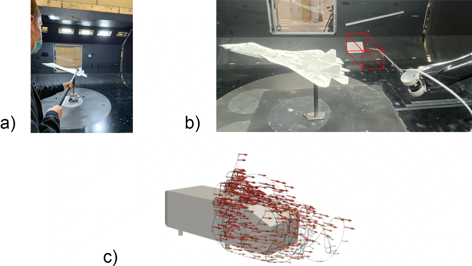
As shown in Figure 1, the project’s output encompasses a human-guided probe solution and a robot-guided solution. While the latter has more accurate probe movement, the former is useful within the augmented reality setup that enables a real-time 3D visualization of the reconstructed flow field (see video below). 

Project goals

We wanted to provide an active learning process, including a sampling strategy and a regression method, which aims to reduce the measurement time, maximize the knowledge gained, and reconstruct the flow field based on the collected data. This task involved multiple scientific challenges.

• As only sparse measurements were available, the flow field reconstruction used a regression model, which had to be powerful enough to interpolate within a large 3D target domain.
• The approach used must be tractable in real-time to provide flow field estimates at any time and at any location. This was essential for optimizing the probe trajectory and enabled the user to visualize the 3D reconstruction of the flow field.
• Capturing the mean value of the flow field (pressure and velocity) at a given location is difficult when the turbulence amplitude is high. Hence, we had to oversample in the high-variance regions to capture the rapid changes in the flow field. In contrast, we undersampled where the flow field was mostly unobstructed. This required uncertainty quantification in the target domain.
• The sampling strategy has to be adapted according to the updated uncertainty estimate.
• The algorithm has to be implemented in a suitable computing infrastructure to enable the real-time feedback loop between the data acquisition and the statistical model.

To address these challenges, we broke down the problem into two main statistical questions:

1. Regression task: Given a set of sampled data points (location, pressure, velocity), how could we reconstruct the flow field (pressure, velocity) over the whole target domain?
2. Sampling strategy: Given a set of sampled data points (location, pressure, velocity) and a flow field estimation, how should the next sample location be chosen?

We outline that our approach’s output encompasses two regression models for the pressure field (and its fluctuations) and the velocity field respectively. The former is exploited to guide the probe within the second phase of the sampling strategy. We estimate the turbulence from the fluctuations of the pressure.

Regression model 

The regression task aimed to recover the functional dependency f such that y = f(x) + ε  where y is the observed pressure (or velocity) at location x in the target domain and ε is white noise with variance r(x) which corresponded to the turbulence amplitude at location x. The function r modeled the uncertainty of the problem. Our approach relied on Gaussian Processes (GPs) that enabled us to estimate both f and r given a set of collected data points. It differs from a standard GP by implementing solutions for three key aspects:

• Heteroscedasticity: We assumed that the GP’s noise variance is spatially dependent. Using an Expectation-Maximization procedure like Kersting et al. (2007), our approach estimates the pressure (velocity) and turbulence. 
• Sparsity: Leveraging the approach introduced by Lázaro-Gredilla et al. (2010), we constructed a GP for which the computation of the mean and the variance is tractable for a large number of data points.
• Nonstationary kernels: The model improved its flexibility because we relaxed the standard assumption of stationary kernels and adapted it to samples that are not uniformly distributed over space.

The difficult task was to find a solution that combined these crucial aspects into a single model, accounting for the flow field’s nonlinear nature and the sampling’s nonuniformity. Furthermore, our approach is tractable in real-time, i.e., we can provide an estimate of the flow field and turbulence field at any location and at any time. Figure 2 shows the reconstructed flow field and turbulence field obtained by employing our GP regression on data collected in the wind tunnel at ETH Zurich.

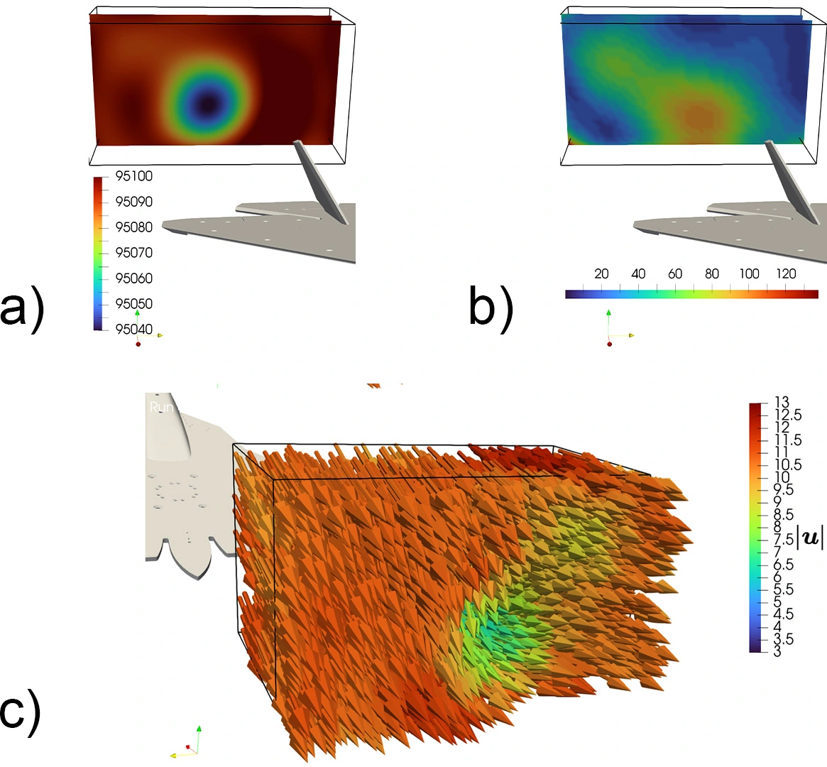
It is worth noting that we only captured the turbulence of the pressure field, which corresponds to the amplitude of the fluctuations of the pressure at each location of the target domain. This could also be done for the turbulence of the velocity field. Although we can extract the same uncertainty, it is computationally easier to reconstruct the turbulence from the scalar pressure field than from the 3D velocity field.

Sampling strategy

We introduced a sampling strategy to guide the probe to reduce the overall wind tunnel time. The strategy consisted of two distinct phases: an exploration phase that includes some randomness and an exploitation phase that tracks the estimation error.

Exploration phase: Thanks to fluid dynamic theory, we know that low-pressure vortices correspond to high-amplitude turbulences. Therefore, without any prior knowledge of the object geometry (aerodynamic properties), we started oversampling areas of low pressure with randomness. These locations gave us a basis for exploration and are relatively easy to sample. Sequentially exploring these regions also forces the algorithm to discover the flow's steeper gradients and, therefore, regions that tend to have high variance (turbulence). Our algorithm is inspired by the Metropolis-Hastings algorithm [7].

Exploitation phase: Once we had collected enough samples from the exploration phase, we leveraged the uncertainty estimate to guide the probe. Hence, we successively move the probe towards the location by maximizing the posterior variance of the estimated turbulence and the posterior variance of the pressure (velocity) field. This ensures the convergence of the estimation at the end of the measurement.

We emphasize that both phases oversample in low-pressure areas but with different objectives. While the first phase aims to discover the low-pressure vortices by exploring the target domain, the second one aims to refine the flow field estimation by guiding the probe toward the most uncertain locations, which are identified using the GP regression.

Results

While we can show the efficiency of our approach on benchmark examples, assessing the quality of our approach in real experiments is difficult as we do not have access to the ground truth. However, we can qualitatively compare the presented approach with the current practice of “Traverse Sampling”. When traversing, the sampling equipment moves along a predefined grid in a continuous fashion. Figure 3 shows the probe trajectory of both sampling strategies and the corresponding reconstructed velocity field. One can observe that the reconstructed velocity field obtained with Smartair is smoother and, according to fluid dynamic theory, captures the region of interest more accurately, in this case, the wingtip vortex. This is due to the extensive measurement time spent on sampling the dynamic regions of the field.

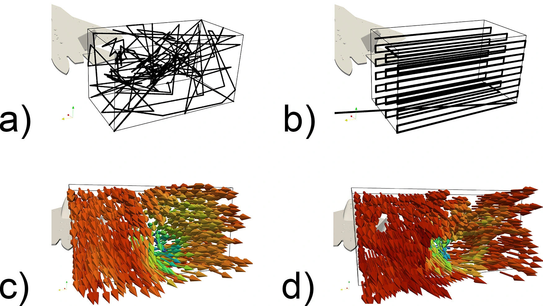
Further experiments show that Smartair gets the same accuracy as traverse sampling with 20% less measurement time. The following movie shows Smartair in use in the wind tunnel facility at ETH Zurich. The two phases of the sampling strategy are visible: the first phase explores the target domain with randomness, while the second focuses on the area that corresponds to the wingtip vortex, which is the most uncertain region of the target domain according to the GP regression. We can also observe the real-time updates of the visualized flow field within the augmented reality setup.

Video 1: Smartair Measurements at ETH Zurich.

Smartair is implemented in both wind tunnels at ETH Zurich and the California Institute of Technology, which resolves the last computing challenge.

Conclusion

We have developed Smartair, a system that rivals the accuracy of conventional wind tunnel measurement techniques. Its autonomous sampling strategy and regression modeling require minimal prior flow field knowledge. Simply place the object in the wind tunnel, and the active learning algorithm begins. Smartair measures the target domain until a predefined time limit or model certainty is reached, saving costs, energy, and human resources. To the best of our knowledge, this is the first machine learning based solution to measure flow fields using wind probe data, and its approach has the potential for broader flow field analysis.

More details about the presented regression model and the experimental setup can be found in Humml et al. (2024) (https://arc.aiaa.org/doi/abs/10.2514/6.2024-1382). Feel free to reach out if you are interested in the project.

Co-authors

• Julian Humml, Center for Autonomous System and Technologies, The California Institute of Technology, formerly at the Institute of Fluid Dynamics (IFD), ETH Zurich
• Fernando Perez Cruz, Swiss Data Science Center, ETH Zurich
• Thomas Rösgen, Institute of Fluid Dynamics (IFD), ETH Zurich

References

1. Humml J., Cohen V., Perez-Cruz F., Gharib M., Rösgen T. Augmented Reality Guided Aerodynamic Sampling, AIAA SCITECH 2024 Forum. https://doi.org/10.2514/6.2024-1382
2. Blazek, J. Computational fluid dynamics: principles and applications. Butterworth-Heinemann, 2015. https://doi.org/10.1016/C2013-0-19038-1
3. Schütz, T. Hucho - Aerodynamik des Automobils: Strömungsmechanik, Wärmetechnik, Fahrdynamik, Komfort. Wiesbaden: Vieweg, 2013. https://doi.org/10.1007/978-3-8348-2316-8
4. Tropea, C. Springer handbook of experimental fluid mechanics. Springer, Berlin, 2007. https://doi.org/10.1007/978-3-540-30299-5
5. Lázaro-Gredilla, M.,Quiñnero-Candela, J.,Rasmussen, C. E., and Figueiras-Vidal, A. R. Sparse spectrum gaussian process regression. Journal of Machine Learning Research, 11(63):1865–1881, 2010. https://doi.org/10.5555/1756006.1859914
6. Kersting, K., Plagemann, C., Pfaff, P., and Burgard, W. Most likely heteroscedastic gaussian process regression. In Proceedings of the 24th International Conference on Machine Learning, ICML ’07, pp. 393–400, 2007. https://doi.org/10.1145/1273496.1273546
7. Chib, S., Greenberg, E. Understanding the Metropolis-Hastings Algorithm. The American Statistician, Vol. 49, No. 4, pp. 327-335, 1995. https://doi.org/10.2307/2684568